ME 50: Experiments and Modeling in Mechanical Engineering
ME 50 is a two-term course dedicated to the analysis of fluid flow around obstructions and of solid materials under load, both through simulated models and with physical experiments.
The course's lab modules were incredibly useful in introducing me to ANSYS Fluent and Mechanical, and the use of experimental water tunnels, universal testing machines, strain gages, and DIC analysis. I also developed my report-writing skills: data and analyses were either written in the AAIA Journal format or organized in technical PowerPoint presentations.
The material below is a very small sampling of the contents of these reports:

One of the CFD assignments involved modeling a NACA 0012 airfoil at a 6-degree angle of attack against 1 m/s fluid flow. Various models were used: one with inviscid assumptions and two laminar models (one steady and one transient). I also explored the effect of mesh granularity by running simulations with the (very coarse!) default mesh, and then several finer meshes. From the simulation data, reported values for lift and drag were collected and discussed.


The first equation is the NACA 00XX equation. However, this equation does not close the trailing edge of the airfoil; i.e. at x = c, yt does not shrink to 0. The sharp trailing edge is important for the CFD simulation, so the last coefficient will be modified to satisfy these conditions. Setting x = c and solving yt = 0 for the last coefficient (formerly 0.1015) gives a value of 0.1036, shown in the second equation.
I wrote a brief MATLAB script to write the airfoil coordinates into a text file readable by ANSYS. A few more lines allowed me to plot the boundary layer of the airfoil, pictured below/to the right:
t = .12;
n = 200;
c = 10.16; %chord length in cm
Re = 101125;
x = linspace(0, 1, n);
modified_coeff = (0.2969 - 0.1260 - 0.3516 + 0.2843);
yt_pos = t/0.2*(0.2969.*sqrt(x) - 0.1260.*x - 0.3516.*x.^2 ...
+ 0.2843.*x.^3 - modified_coeff.*x.^4) + x.*(4.91/sqrt(Re));
yt_neg = -1 .* yt_pos;
M = [horzcat(ones(n, 1), transpose(1:n), ...
transpose(c*x),transpose(c*yt_pos), zeros(n, 1)); ...
horzcat(ones(n, 1), transpose(n:2*n-1), ...
rot90(c*x),rot90(c*yt_neg), zeros(n, 1)); [1 0 0 0 0]];
M(2*n, :) = [];
M(n+1, :) = [];
fileID = fopen('C:\Users\Galilea\Documents\NACA0012_BL.txt', 'w');
fprintf(fileID, '%5d %5d %10f %10f %5d \n', M');
fclose('all');

Boundary layer for Re = 101,125 plotted over a mesh of the airfoil
FEA - ANSYS Mechanical
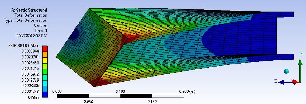
Static structural deformation of a cantilevered I-beam under deflection and torsion
Above is an image from a set of simulations of a cantilevered I-beam with an end cap. The following free body diagram describes the loading situation (an off-centered downward force inducing deflection and torsion) for the static structural simulation.
I also performed a modal analysis, and a transient analysis whose time steps were determined based on the modal analysis. The first three modes of the beam are pictured below.
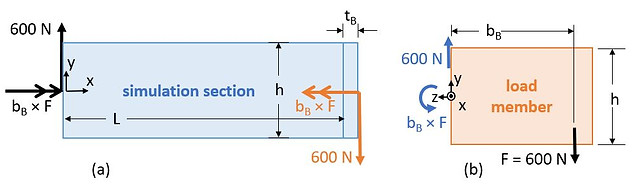
Loading conditions for the static structural analysis. Only the simulation section was modeled in ANSYS; the effective forces on the simulation section, based on the forces on load member, were input into the simulation as boundary conditions.

The first three modes of the I-beam with cap (weak-axis bending, strong-axis bending, and torsion)
Note that these simulations were performed under conditions that would only induce elastic deformation, so there was no need to inform ANSYS of a kinematic hardening curve in the plastic regime, as was necessary in another FEA project for the course.
Particle Image Velocimetry
Mechanical engineering undergraduates are lucky enough to have an undergraduate teaching laboratory complete with a water tunnel, an ADMET universal testing machine, and other important instruments for exclusive teaching use. ME 50 experiments are performed in this lab.
The water tunnel is 20 cm × 20 cm × 200 cm, with transparent sides and underside, as pictured. Through it flows an (initially) laminar flow of water seeded with 10 µm glass hollow spheres. Flow speed is maintained by a 7.5 horsepower pump capable of reaching 60 Hz. The pumping frequency is widely adjustable to produce different water flow rates within the tunnel; the approximate relationship between these parameters has been calibrated and tabulated for easy reference in the lab.
The flow around an object in the tunnel can be measured with Particle Image Velocimetry (PIV). PIV is a method of imagining the velocity field of a fluid by seeding the fluid with tiny particles that reflect laser light. The laser shines a sheet of light to present a two-dimensional space for photography by a CCD camera. The laser and camera are synchronized such that it is possible to pulse the laser and take two photographs with a very short time interval between them (the timed pulse of the laser is critical in navigating the limitations of the memory read-out time of the camera). Computer software discerns the movement of the particles between these image pairs, outputting a velocity vector field, or a series of velocity fields over time if multiple image pairs are taken.

The water tunnel experimental set-up


The images above describe the second ME 50 laboratory experiment performed with the water tunnel: the flow through a turbofan engine model. What follows are some of the key analyses of the data collected.
Data upstream was taken primarily to measure the actual velocity of the incoming flow and various pump speeds, as opposed to the nominal velocity reported by the water tunnel manufacturers. The bulk of the analysis was performed on downstream data.
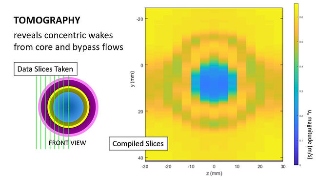
This image is a time-averaged map of the flow downstream of the engine model. We can see the core and bypass flows exit the model separately but merge further downstream in the model's wake.


These are two other ways of visualizing the wake of the engine model: above, the velocity of the flow at a certain radius from the model's axis of symmetry is normalized with respect to the incoming fluid flow.
The annular pattern of the wake is depicted via the compilation of tomographic slices.
These plots and contours were created from the data using the PIVMat toolbox for MATLAB.
Strain Gages
These labs concerned the proper use of, and theory behind, the indispensable strain gage. Rosette gages were used to comprehensively measure planar strain on the surfaces to which they were glued. Note that all of these experiments kept the specimens in the elastic regime.
Four-Point Bend
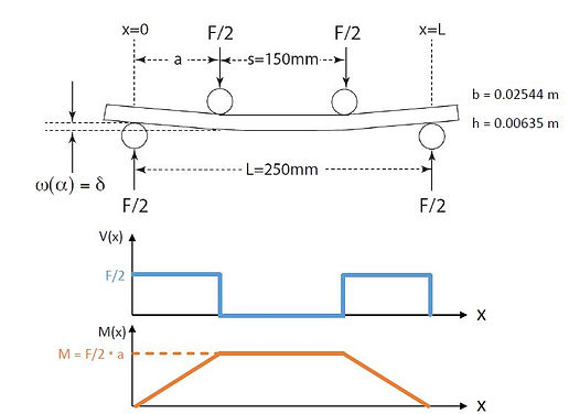
The accompanying figure depicts a classic four-point bending scenario, and its associated shear and bending moment (pure bending between the middle rollers!). This was set up in the ADMET frame with a solid, rectangular prismatic beam of aluminum alloy 6061-T6.
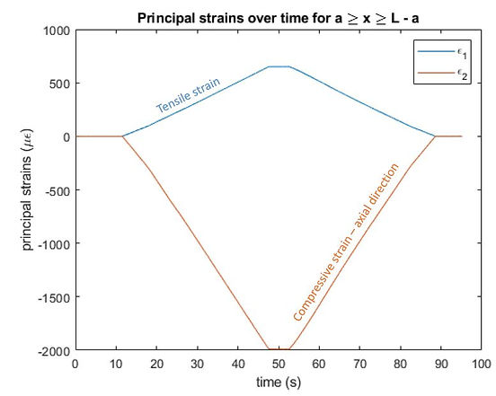
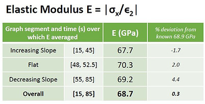
A strain gage was glued to the beam in the a < x < L - a (i.e middle) region, and the principal strain equations were used to general the graph below. Note that the magnitude of the compressive strain is much greater, as expected, and occurs in the axial direction.
By considering the known force applied by the ADMET, we experimentally determined the elastic modulus of the material, and determined Poisson's ratio! The results were very close to the accepted value for 6061-T6.

Cantilever Vibration
A thin, rectangular aluminum cantilever was flicked to induce vibration; a fast Fourier transform of strain gage measurements identified its modal frequencies. Note that only one grid of the strain gage was necessary to collect this data --- but selecting the one most closely aligned with the length of the cantilever gave the cleanest results! The percent error is based on the modal frequencies calculated via formula based on the beam geometry.

Digital Image Correlation
2D digital image correlation (DIC) using the open-source MATLAB program Ncorr enabled analysis of an aluminum alloy 6061-T6 dogbone with a hole in the center under tension in the ADMET universal testing machine. Note that the specimen stayed in the elastic regime.
The correlated images produced U- and V-displacement plots we differentiated with several different strain radii to determine the strain experienced by the dogbone. With some trial and error we found the optimal strain radius to be 9 pixels, which resulted in a stress concentration factor around the hole of 2.36, very close to the accepted 2.35 based on its geometry.


We also examined the precision of DIC by correlating images of an unmoved dogbone, and of a rigidly translated dogbone, and the effects of using static images vs. frame-averaged videos for the image pair. Interestingly, the unmoved dogbone DIC had a noise floor more than 100 times lower with the frame-averaged pair than the static pair, but the rigidly translated dogbone saw a less than 50% decrease in noise between the frame-averaged image pair and static image pair. Regardless, even the highest noise floor was 16.67 microns, small enough to preserve our confidence in the tensile test data.